September 20th, 2016
Pavel Shevchenko

PSCAN2
Superconductor Circuit Simulator

Introduction.

PSCAN2 is a superconductor circuit simulator, based on ideas and experience from development of PSCAN, PSCAN96, and Julia simulators, written by Pavel Shevchenko. It is implemented as a Python module, which can load the circuit netlist, circuit parameters, and description of expected circuit behavior, and when perform transient simulation of the circuit. There are functions to run circuit simulation, calculate margins or circuit parameters, and optimize circuit parameters.
For any questions, please call Pavel Shevchenko: pscan2sim@gmail.com

Circuit netlist.

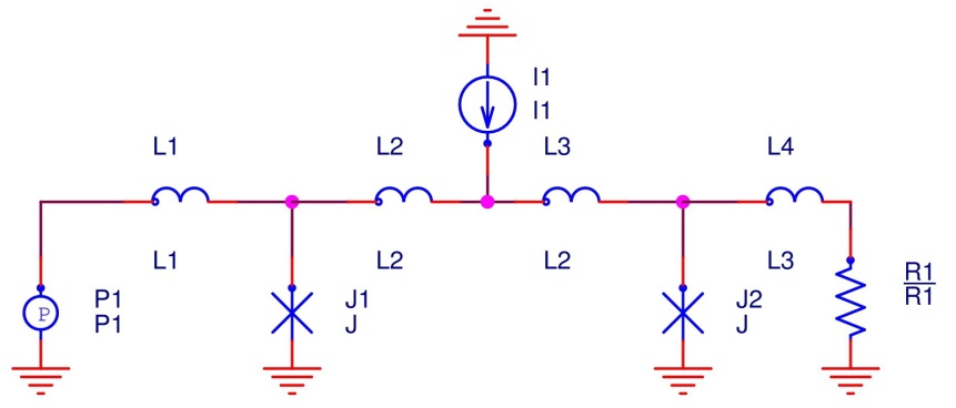
PSCAN2 accept circuits in subset of standard SPICE format. For example, circuit netlist for transmission line will look like this:

Figure 1: Transmission line

R1 1 0 R1

L1 2 n3 L1

L2 n3 n4 L2

I1 n4 0 I?

L3 n4 n5 L2

L4 n5 1 L3

P1 2 0 P1

J1 n3 0 J

J2 n5 0 J

.END

Each line, describing the element, has a format:
<element_name> <node_1> …<node_n> <element_model>
Element’s type defined by the first letter of its name:
‘L’ – inductor
‘R’ – resistor
‘C’ – capacitor
‘I’– current source
‘P’ – phase source
‘U’– voltage source
‘J’ – Josephson junction
‘M’ – mutual inductance
<node_1> …<node_n> are the nodes, element is connected. Nodes can be numbers or identifiers. Node number 0 is a special node, representing connection to the ground.

Element’s models define simulation model, used during numerical simulation of the circuit. For all elements, except Josephson junctions and transformers, model is just an expression. For Josephson junctions it should be expression rsj(Ic, Rn, C), which is a RSJ model with critical current Ic, normal resistance Rn, and capacitance C. For mutual inductance model should be llm(L1,L2,M), where L1 – name of the primary winding inductor, L2 – name of the secondary winding inductor, and M – is the mutual inductance. L1 and L2 inductors should exist in the circuit.

For convenience, PSCAN2 translate element’s models according to the user defined rules. For example, inductance model in the form ‘L?’ or ‘?’ will be converted into expression <name>*X<name>*XL. So, for inductance L2, it will be L2*XL2*XL. For Josephson junctions, model in the form ‘J’ or ‘J?’ will be converted into RSJ(<name>*XJ, 1/<name>, <name>)

PSCAN2 fully supports hierarchical SPICE format. Name of the hierarchical element in the netlist starts with the letter ‘X’, and has the form: X<name> <node_1> … <node_n> <circuit_name>
where <name> is the name of the subcircut instance, <node_1> … <node_n> connected nodes, and <circuit_name> is the subcircut name

Circuit definition file.

Figure 2: Not circuit

In addition to the definition of circuit structure in the netlist, there is definition of crcuit’s parameters and description of its behavior in the circuit definition file. Circuit definition files have extention “.hdl”, and there are separate file for each subcircuit in the circuit, including a root circuit. For example, hierarchical test ‘not’ circuit:

should have definitions for the root circuit, not1, stdin, stdout, and jtl circuits.

Circuit definition has the following form:

circuit <name>()
{
parameter
<param1> = <pval1>,
…
<paramN> = <pvalN>;

external
<external1> = <extval1>,
…
<externalN> = <extvalN>;

internal
<internal1> = <intexp1>,
…
<internalN> = <intexpN>;

value
<value1> = <valexp1>,
…
<valueN> = <valexpN>;

freeze
<jname1>,…,<jnameN>;

rule <rname1>(<init_expr>)
<expr1>,
…
<exprN>;

…
}

<name> - is the circuit name.

parameter - is the definition of circuit parameters. Parameters will have floating point values and can be used in element’s models. They will have the SAME value in all instances of particular circuit. For example, if parameter J1 in JTL circuit will be changed, it will change in all instances of JTL circuit

external - is the definition of circuit external parameters. External parameters will have floating point values and can be used in element’s models. But, unlike parameters, they can have DIFFERENT values in different instances of a circuit. For example, external parameter XJ1 in JTL circuit MTL1 can have different value from the value of XJ1 external parameter in circuit MTL2.

internal - is the definition of circuit internal parameters. Internal parameters defined by floating point expression and can be used in element’s models. Different instances of same circuit can have different values of the same internal parameter. They can depend on current simulation time, and there is one predefined internal parameter ‘tcurr’, which is a current simulation time. But, they cannot depend on phases, currents, or voltages across circuit elements or nodes.

value - is the definition of circuit value parameters. Value parameter defined by floating point expression and can depend on simulation time, phases, currents, or voltages across circuit elements or nodes. But, they CANNOT be used in circuit element’s models. Different instances of same circuit can have different values of the same internal parameter.

freeze - is the declaration of “frozen” Josephson junctions. Such junctions will be ignored during SFQHDL simulation of the circuit. So, switching of “frozen” junctions will not generate an error

rule - is definition of SFQHDL rule, describing expected behavior of the circuit. Rule has a name, <init_expr> expression, which activate the rule when equal to True (any non-zero value). After rule is initialized, it will check sequence of expressions <expr1> … <exprN> for True value one after another, until the last expression will be True. After that, rule will ‘deactivate’, and can activate again. All rules are processed in parallel on each circuit simulation time step. There are two special functions inc(<jname>) and dec(<jname>), which became True during one time step, when number of flux quanta increases/decreases by one on particular Josephson junction. When SFQHDL simulator waits for inc() or dec() function to become True in one of rules, switching of that particular junction do not generate an error. If one of the circuit junctions switched and SFQHDL simulator do not anticipate it in one of the active rules, it means that circuit do not works correctly.

For example, circuit definition file for the not circuit on Figure 2:

circuit testnot()

{

INTERNAL

tp=tseq/4,

p1=0.85+psfq(tseq+tp,4,2*tp),

p2=0.85+psfq(tseq+tp,4,tp)+psfq(tseq+tp,4,3*tp);

rule m1go( inc(p1) )

set(m1.1);

rule M1MTL1( get(m1.2) )

set(MTL1.1);

rule m2go( inc(p2) )

set(m2.1);

rule M2MTL2( get(m2.2) )

set(MTL2.1);

rule MTL3M3( get(MTL3.2) )

set(M3.1);

}

Here we have definition of internal parameters p1 and p2 for phase sources, generating input pulses for the tested not circuit.

Also we have several rules, describing testnot circuit behavior. For example, rule m1go will activate when phase generator p1 produces pulse – switches. After that, function set(m1.1) will set state variable on the node connected to the node 1 of the circuit m1(stdin). Rule M1MTL1 will activate when circuit m1 set state on the node 2, function get(m1.2) read it, and set state on the node 1 of the JTL circuit MTL1.

Now, let’s look at the circuit definition file for the stdin:

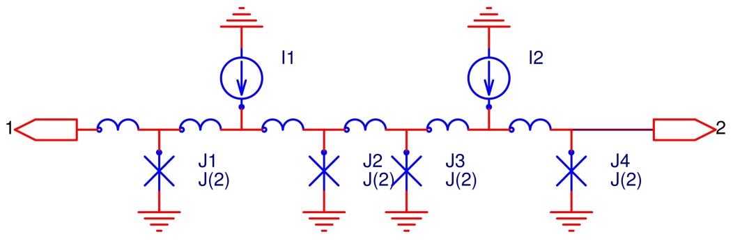
Figure 3: Stdin circuit

circuit stdin()
{

freeze j1;

rule input(get(1))
[inc(j2),inc(j3)],
inc(j4),
set(2);

}

Here we cannot predict when exactly junction j1 will switch, so we declare it ‘frozen’, and completely ignore its behavior.

Rule input will activate, when set() function will be called on node 1 in some other circuit. Junctions J2 and J3 can switch almost simultaneously, so we use a sequence expression […], which will check all expressions, enclosed in square brackets in ANY ORDER in time. At the end of the rule we will set state on the node 2, so get() function on that node will return True.

Global parameters and internals.

Global parameters or internals can be declared outside of any circuit. They are visible in all circuits and parameters declared inside circuit definitions cannot have similar names.

Expression syntax.

Numeric constants. Example: 1.2
String constants. Example: “var1”
Identifiers. Example: xj1
Operators in order of precedence:
- ‘-‘ - unary minus
- not,! - unary logical not
- * - binary multiply
- / - binary divide
- + - binary plus
- - - binary minus
- < - less than
- <= - less or equal
- > - greater than
- >= - greater or equal
- eq, == - equal
- ne, != - not equal
- and, && - logical and
- or, || - logical or
Functions:
- p(<node>/<element>) – phase on the circuit node or across element
- v(<node>/<element>) – voltage on the circuit node or across element
- i(<element>) – current through the element
- n(<jelement>/<pelement>) – number of flux quanta passed through Josephson junction or phase source
- inc(<jelement>/<pelement>) – returns true at the time step when number of flux quanta increases across Josephson junction of phase source
- dec(<jelement>/<pelement>) – returns true at the time step when number of flux quanta decreases across Josephson junction of phase source
- psfq(<period>, <duration>, <start>) – generate 2π pulses, with duration <duration>, starting at time <start>, with period <period>
- min(<args>) - returns minimal value of arguments
- max(<args>) - returns maximal value of arguments
- set(<node>) – set node’s internal variable to true, during the next time step
- get(<node>) – returns value of node’s internal variable
- exit(<message>, <condition>) – exit rules execution with error message <message> if <condition> is non-zero (true). Used in rules to abort circuit simulation upon some condition. For example:
  exit('Wrong state', sts1 == 2 and n(j1) > n(j2))
- print(<v1>, ….) – print string representation of argument values on the screen, during rules execution. Always returns true. For example:
  print('State value stst1=', stst1)
- freeze(<jname1>, …) – place junctions into the set of “frozen” junctions. Switching of such junctions will be ignored during circuit simulation. Always returns true. For example:
  freeze(j1, j2)
- unfreeze(<jname1>, …) – remove junctions from the the set of “frozen” junctions. Always returns true. For example:
  unfreeze(j1, j2)
- integrate(<exp>) – Return integral over time from 0 to current simulation time of value of expression <exp>. For example:
  integrate(v(j1)) – should be equal to phase over junction j1
- all functions from the Python’s math module. For example:
  sin(0.01*tcurr)
Special operators, which can be used only in rules:
- <var>=<value> - assignment operator. Assign value to the parameter or external parameter. Always returns true. Example: xst = 1
- [<exp_1>,…, <exp_n>] – sequence operator. Equal to true if all expression in brackets was equal to true at some point of time. In can be used in rule to describe situation, when we do not know sequence of Josephson junction switches. For example: [inc(j1),inc(j2)].

Parameters value file.

In order to simplify saving and loading of circuit parameters PSCAN2 supports parameters values files. Those files have extension “.par” and coexist along with circuit definition files. Format of those files are very simple, each line consists of pair:
<parameter> <value>
where <parameter> is the name of circuit parameter and <value> is floating point value of that parameter.
After PSCAN2 loaded circuit definition file with name <circuit>.hdl it will look for parameters file with the name <circuit>.par and if such file exists will load parameters values from it

Python interface.

PSCAN2 implemented as a Python module pscan2 and include following functions:

initialize(<args>) – initialize PSCAN2 and load circuit netlist and definition files
<args> is the array of arguments, where the last argument is the name of root circuit and base name of the circuit netlist file (full name of the file will have “.cir” extension appended). All previous arguments, if existed, will be names of circuit definition files, preloaded into memory. After loading netlist file, PSCAN2 will try to load circuit definition files used in the netlist. If circuit definition was preloaded, it will use that definition, otherwise it will try to load corresponding “.hdl” file.

find(<name>[, <type>])
Find objects in circuit hierarchy by name.
<name> is a hierarchical name of object. For global parameters or global internals it is just a name. For example: find(“XI”). For parameters in circuits, full_path should be circuit name, "." and parameter name, for example find("jtl.p1", "p"). For the objects in root circuit, name should start with “.”. For example, find(“.XJ1”). For objects on deeper levels of hierarchy, name should contain all subcurcuit instances, separated by “.”. For example: find(“.m1.jtl1.XJ1”). For elements, nodes, and rules "." in the beginning of name should be removed, so junction J1 in root circuit will have path "J1". For junction in circuit jtl1 path will be "jtl1.J1"
<type> is a type of object to find:
'e' – circuit element
'n' – node
'p' - parameter or external. Default value
'v' - internal or value
'r' - rule
Function will return instance of found object, or raise exception, if object was not found

param_find(<circuit_name>, <parameter_name>)
Find parameter <parameter_name> in a circuit <circuit_name>. There is no need to specify full hierarchical path for parameters. They can be found giving only circuit name. Function will return object instance of the parameter, or raise exception.

find_re(<pattern>[, <type>])
Similar to find() function, but returns list of objects, given simple regular expression as element name. It uses Python module fnmatch and support following special symbols in pattern:

Pattern	Meaning
*	matches everything
?	matches any single character
[seq]	matches any character in seq
[!seq]	matches any character not in seq

<type> is a type of objects to find, the same as in find() function
Function will return list of found objects. If no objects match the pattern, list will be empty.
For example: find_re(“m1.xj*”) will find all parameters in circuit m1, started with “xj”.

param_re(<circuit_name>, <pattern>)
Similar to param_find() function, but returns list of circuit parameters matches simple regular expression, with same syntax as in find_re().
For example: param_re(“not1”, “j*”) returns all parameters in circuit “not1”, started with character “j”.

simulate(<tseq> [,print_messages = False, pretty_print = False])
Simulate circuit and test SFQHDL rules.
<tseq> is the maximal simulation time. If, during simulation, some junction will switch, but it was unexpected (there are no any rule, which is waiting for its switching in inc() or dec() expression), simulation will stop. If print_message argument is True, there will be trace of rule execution during simulation. If pretty_print argument is True, rule traces will be printed in nice ascii pseudo-graphical form. If there was no any unexpected Josephson junction switched during simulation and there are no any active rules left, function will returns True, otherwise False

margins(<parameter>, <tseq>[, messages_level=0, max_margin=0.4])
Calculate operating margins of parameter.
<parameter> - name of parameter or circuit parameter or external object instance, obtained with functions find() or param().
messages_level argument set amount of printed messages:
0 – no any messages
1 – basic messages about calculating <parameter> margins
2 – all messages, including rule’s execution traces, during circuit simulations
max_margin – is the maximal expected value of parameter margins. For example, if parameter value is 1.0, max_marging equal to 0.4 means that circuit will correctly works for parameter range from 0.6 to 1.4.
Function will returns list of two elements: left and right margins, or list of two None objects, if circuit does not work with initial value of parameter.

save_parameters(<circuit_list>) – save circuit parameters into parameters values files.
<circuit_list> is a list of circuit names to save. For each circuit from the list parameters files <circuit>.par will be created.

load_parameters(<circuit_list>) – load circuit parameters from parameters values files.
<circuit_list> is a list of circuit names to load parameters. For each circuit from the list, if parameters files <circuit>.par exists, it will be loaded.

ivcurve(<xpar>, <xmin>, <xmax>, <dx>, <xback>, <yexpr>, <yeps>, <twait>, <tmin>, <tmax>)
– calculate iv-curve.
<xpar> - parameter to change. Can be found by function find(). For example find('.i1', 'p')
<xmin> - minimal value of parameter
<xmax> - maximal value of parameter
<dx> - step for parameter's changes
<xback> - if False parameter will be changed from <xmin> to <xmax> with step <dx>.
if True parameter will be changed from <xmin> to <xmax> and when back to <xmin>
yexpr - expression to average over the time for each value of parameter <xpar>
Can be calculated by function create_expression(). For example create_expression("v(j1)", ".")
<yeps> - relative accuracy to average expression <yexpr> over time
<twait> - wait time between changing parameter <xpar> and starting averaging expression <yexpr>
<tmin> - minimal time to average expression <yexpr>
<tmax> - maximal time to average expression <yexpr>. Even if accuracy is less than yeps averaging will stop.
Function returns list of [x,y] pairs

Circuit parameters optimization.

Optimization of circuit parameters starts with creating Optimizer object, and when calling optimize() method of that object:
opt = Optimizer(<optimized_list>, <change_list>, <tseq>)
opt.optimize()
<optimize_list> is a list of parameters to optimize. Each list item is a list of parameter name or parameter object and required margin.
<change_list> is a list of parameters allowed to change. Each list item can be a parameter name in the format as in function find(), parameter object or list of parameter name or object and min abd max value of parameter.
<tseq> is a maximal simulation time.
For example:

optimized_list = [['xi',0.3], ['xj',0.3], [‘mi.xj1’, 0.3]]

change_list = param_re('not1', 'j*')+param_re('not1', 'i*')+param_re('not1', 'l*')

opt = Optimizer(optimized_list, change_list, 400)

opt.optimize()

will optimize global parameters xi and xj, and parameter xj1 in circuit mi up to 30% margins, changing all Josephson junctions critical currents, all current sources, and all inductances in the circuit not1.

Test vectors.

Test vectors can be used to define input signals during circuit simulation. They should be defined as instances of Python class TestVector and when used in phase generators definition.

Definition of Python class TestVector has form:
TestVector(name, vec, tunit = 20.0, period = 0, repeat = 0, start = 20.0, pulse_duration = 5.0)
where
name – is the name of test vector. If name is not empty string (“”), test vector will be placed in the global test vector table and can be used in circuit.
vec - definition of test vector values. It can be string containing “0” or “1” of vector of 0 or 1. If value is 1 there will be a change of test vector value by 2, if value is 0 there will be no changes
tunit – is a time unit. All changes occurs in the beginning of tunit intervals
period – length of test vector section. If period grater than length of vec parameter, vector will be appended by “0” to the period length
repeat – repeat count. Test vector will be repeated repeat times and when stays constant. If repeat is equal to 0, test vector will repeat indefinetly
start – start time of test vector. All changes in test vector will be at times equal to start + N*tunit
pulse_duration – duration of test vector pulse

Best place to define test vectors is the pscanrc.py file, which will be automatically loaded before loading circuit definition from .cir and .hdl files. For example pscanrc.py file for testnot circuit can looks like:

from pscan2.TestVector import TestVector

tv1 = TestVector("d1", "01", 100.0, 0, 1, 100.0)
tv2 = TestVector("d2", "101", 100.0, 0, 1, 100.0)
TestVector.printAll()

In the first line it import TestVector class definition from pscan2 TestVector module. When it defined two test vectors with names “d1” and “d2”. At the last line it prints global table of test vectors.
In the circuit definition those test vectors can be used as:

INTERNAL

p1=0.85+tvec("d1"),

p2 = 0.85 + tvec("d2");

Appendix A. Elements models.

In PSCAN2, current through different elements defined by the following equations:

Inductor:

$I_{i, j} = \frac{ϕ_{i} - ϕ_{j}}{L}$ , where $ϕ_{i}$ and $ϕ_{j}$ are phases in nodes i and j

Resistor:

$I_{i, j} = \frac{\dot{ϕ_{i}} - \dot{ϕ_{j}}}{R}$

Capacitor:

$I_{i, j} = C * (\ddot{ϕ_{i}} - \ddot{ϕ_{j}})$

RSJ model of josephson junction:

$I_{i, j} = I_{c} * \sin (ϕ_{i} - ϕ_{j}) + \frac{\dot{ϕ_{i}} - \dot{ϕ_{j}}}{R} + C * (\ddot{ϕ_{i}} - \ddot{ϕ_{j}})$
in circuit netlist model call should be rsj(Ic, Rn, C)

RSJN model of Josephson junction:

$I_{i, j} = I_{c} * \sin (ϕ_{i} - ϕ_{j}) + \frac{V_{i, j}}{R} * \frac{{(\frac{V_{i, j}}{V_{g}})}^{n}}{1 + {(\frac{V_{i, j}}{V_{g}})}^{n}} + C * (\ddot{ϕ_{i}} - \ddot{ϕ_{j}})$
where $V_{i, j} = \dot{ϕ_{i}} - \dot{ϕ_{j}}$ , $V_{g}$ - voltage gap, n – positive even number, practically from 6 to 10.

in circuit netlist model call should be rsjn(Ic, Rn, Vg, n, C)

Tunnel model of Josephson junction:
Use Dirichlet series approximation of kernels in tunnel junction model.
In circuit netlist should be tjm(coeff_set_name, Ic, Beta, Wvg, Wvcrat, Wvrrat) where:
coeff_set_name – TJM parameters set name in the file psconfig.py. By default pscan2 has parameter set “tjm1”, provided by Prof. Semenov
Ic – critical current
Beta – parameter beta
Wvg – gap voltage
Wvcrat – Vc/Vg ratio
Wrrat – Rn/Rj ration.
There is simpler substitution model jt(Ic, Beta) which uses “tjm1” coefficients set and global parameters wvg, wvcrat, and wrrat.

Mutual inductance:

$ϕ_{i} - ϕ_{j} = L1 * I_{i, j} + M * I_{k, l}$ $I_{k, l}$

$ϕ_{k} - ϕ_{l} = L2 * I_{k, l} + M * I_{i, j}$
between inductances L1 and L2, connected to nodes i,j and k,l respectively. In that case $I_{i, j}$ and $I_{k, l}$ are independent variables, equal to current from node i to node j, and from node k to node l.